Getting Started
Learning objectives
- Get familiar with the room
- Get familiar with the course mechanics
- Become etherpad and sticky note masters
Orientation to the course
- Setup (as you arrive)
- software installation
- power outlets
- internet access
- Brief introduction of co-instructors
- Restrooms
- Coffee/tea/water/juice
- Code of Conduct
- Territory acknowledgement
- Data Carpentry
- Live coding
- slows the pace
- increasing retention with multiple ways of getting information
- watch my mistakes and how I fix them
- Sticky notes
- Green: I’m finished with the task; I’m ready to move on; Feedback on something that’s going well for you
- Red: I have a question; I’m not ready to move on; Feedback on something we can improve
- Live coding
- Important links
- Introductions
- Name
- Affiliation
- Field of study
- Something you made recently that you’re proud of
- Motivating examples
- This website!
- Where are we coming from and where are we going…
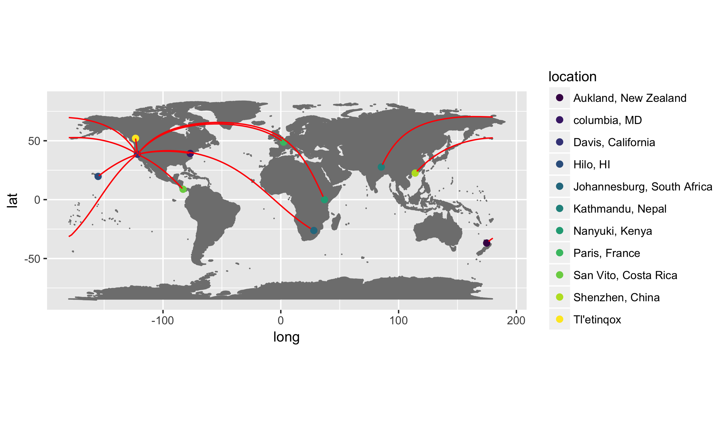
A motivating example…
This is an example R script. Don’t try to take in all the details just yet. Instead, let it wash over you and get a gestalt sense of where we are coming from and where we are headed…
# Load necessary packages
library(tidyverse)
library(viridis)
library(geosphere)
library(ggmap)

# What is the current location of the workshop?
currentLocation_str <- "Davis, California"
currentLocation <- geocode(currentLocation_str)

# Import the data
learners <- read_csv("dc_origins.csv")

# Use the mutate_geocode() function in the ggmap package on that new column to
# add new columns to the dataframe representing the longitude and latitude of
# each learner's hometown as a result of a Google Maps lookup.
# [For instance, if your hometown is "Davis, California", the mutate_geocode()
# function will return -121.7405 in the "lon" column and 38.54491 in the "lat"
# column]
# Remove any rows that fail to geocode. Sorry!

learners <-
  learners %>%
  as.data.frame() %>%
  mutate_geocode(location) %>%
  filter(complete.cases(.))

# Use the gcIntermediate() function from the geosphere package to get points
# representing the Great Circle paths between each learner's hometown and the
# current location of the workshop.
gcPoints <-
  gcIntermediate(p1 = learners[, c("lon", "lat")],
                 p2 = currentLocation[, c("lon", "lat")],
                 breakAtDateLine = TRUE
                )

# Loop through each Great Circle path and assign each a unique identifier. If
# the Great Circle passes the International Date Line, each segment on either
# side of the Date Line needs to get it's own group identifier so it can be
# plotted separately. In these cases, assign each of the 2 segments a unique
# id, then bind the 2 list elements into a single data frame. If the Great
# Circle does *not* cross the International Date Line, add the unique identifier
# and coerce the list element into a data frame (from a matrix). Ensure all
# column names for each list element data frame have the same names.

for (i in seq_along(gcPoints)) {
  currentPath <- gcPoints[[i]]
  if(is.list(currentPath)) {
    currentPath[[1]] <- data.frame(currentPath[[1]],
                                   path = paste0(i, ".1"),
                                   stringsAsFactors = FALSE)
    currentPath[[2]] <- data.frame(currentPath[[2]],
                                   path = paste0(i, ".2"),
                                   stringsAsFactors = FALSE)
    currentPath <- bind_rows(currentPath)
  } else {
    currentPath <- data.frame(currentPath,
                              path = paste0(i),
                              stringsAsFactors = FALSE)
  }
  colnames(currentPath) <- c("lon", "lat", "path")
  gcPoints[[i]] <- currentPath
}

# Combine the list of data frame elements into a single dataframe, since we know
# each list element data frame has the same number of columns and the same
# column names
gcPoints <- bind_rows(gcPoints)

# Create a plot of the locations of each student's email_affiliation on a globe
# by mapping the longitude to the x position on the plot, and the latitude to
# the y position on the plot. Use the borders() function from ggplot2 to
# generate a rough sketch of the land masses on Earth. Color all the points red
# and make them twice as large as default. Ensure that the figure has a 1:1
# ratio between units on the x-axis and units on the y-axis.
dc_origins <- ggplot() +
  borders("world", colour = "gray50", fill = "gray50")  +
  geom_point(data = learners, aes(x = lon, y = lat, color = location), size = 2) +
  scale_color_viridis(discrete = TRUE) +
  coord_equal() +
  geom_line(data = gcPoints, aes(x = lon, y = lat, group = factor(path)), color = "red")

# Visualize the plot that we just made
dc_origins

# Save the plot we made as a .png file to our working directory while
# specifiying its height and width
ggsave(plot = dc_origins,
       filename = "dc_origins.png",
       device = "png",
       units = "cm",
       width = 20,
       height = 12)
This code produced the below figure for an example dataset.